Visualisation of geometry and data

When it comes to understanding one’s Geant4 geometry or data, it is very useful to be able to launch a 3D visualisation of the volumes and tracks in question. While such visualisations lack the precision and number crunching performance of a carefully written data-analysis, they instead have the potential to provide quick and instant feedback on a setup, in a manner that is very intuitive to the human developers and consumers of a simulation project.

In dgcode, we facilitate the usage of two options for 3D visualisations out of the box: the one included in Geant4 itself, and our own custom application.

Custom 3D Viewer

In dgcode, we provide a custom OpenSceneGraph-based 3D visualisation tool which can be used to visualise both simulation geometries and data. Despite being a bit rough around the edges (for instance it could use a better name than “CoolNameHere”), it has already been highly useful for a lot of work so far.

Geometry visualisation

Simply supply the --viewer flag to any simulation script to launch our viewer. If for instance you have just started a new simulation project named TriCorder, the command to use will be:

$> sb_tricorder_sim --viewer

And the viewer is launched:

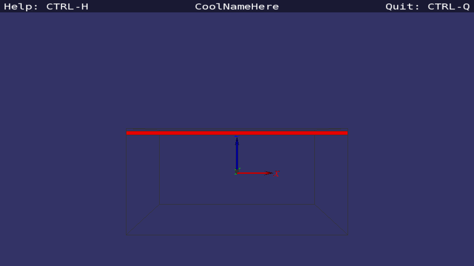
Warning

There is a known issue on macOS where the viewer will either crash or only use part of the graphics window. There is a workaround described in this comment.

Grab the mouse and change the view as you see fit:

• Left-click + move: rotate view.

• Middle-click + move: pan view.

• Scroll wheel or right-click + move: zoom view.

• Right-click or left-click+S on a volume: center view on a selected point on the geometry.

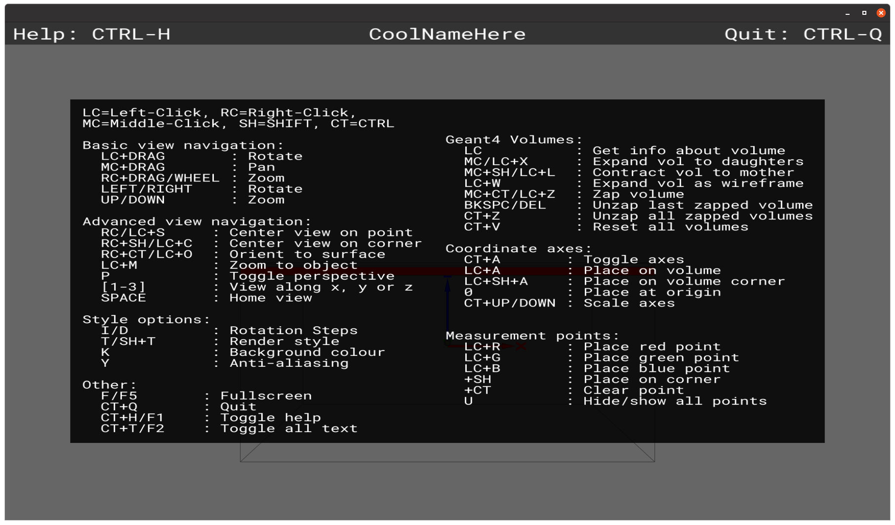
There are many more options for how to interact with a geometry, change display style, add measurement points and coordinate axes, and so on. Hit F1 or Ctrl+H to see them summarised:

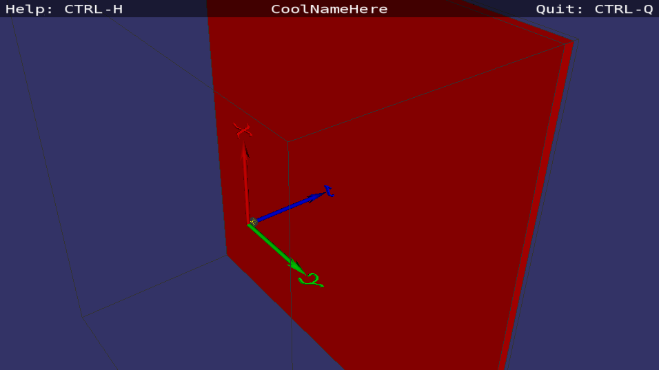
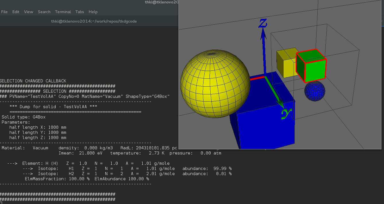
In particular, when a Geant4 geometry is hierarchical, it is of great value to be able to “open up” a volume to see the volumes inside it:

• Left-click on a volume: get information about geometry and material printed in the terminal.

• Middle-click on a volume: open it up (i.e. make it invisible) and display daughters (does nothing if it has no daughter volumes).

• Left-click+W on a volume: open up the volume by rendering it with a wireframe rather than simply making it invisible (if it has no daughter volumes, it will simply toggle the volume in and out of wireframe).

• Shift+middle-click on a volume: close the containing volume (i.e. display the containing volume normally, and hide the volume itself and it’s “siblings”).

Simulated data visualisation

It is pretty bare-bones at the moment, but the viewer also offers a non-interactive view of simulated tracks along with the geometry. To get it, one must supply the --dataviewer flag instead of the --viewer flag, and as usual, use the -n (or --nevts) flag to choose the number of events to be simulated. So, still using the TriCorder example from here, we can run:

$> sb_tricorder_sim -n100 --dataviewer

Gives the view (nb. the coordinate axes were hidden with ctrl+A since they were in the way and the spherical sample volume was turned into wireframe with a left-click+W, in order to be able to see the tracks inside it):

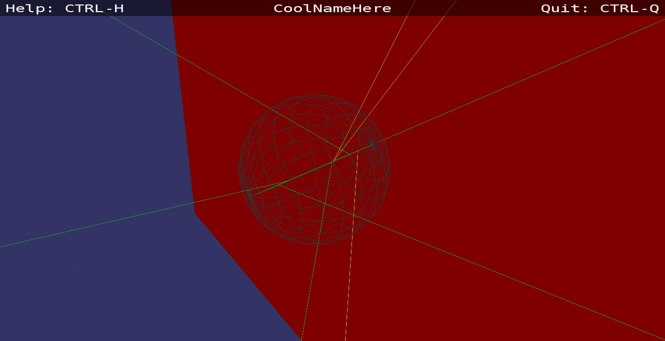
A pencil-beam of neutrons (green) are generated at the left side of the sample, headed to the right. Notice how roughly 5 of the 100 neutrons had an interaction in the sample, leading to both scatterings and generation of gammas (yellow). For fun, here are instead 10000 neutrons:

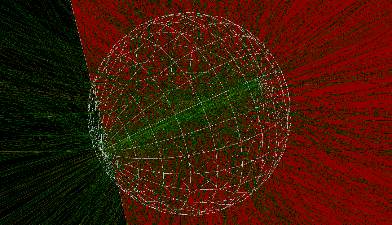
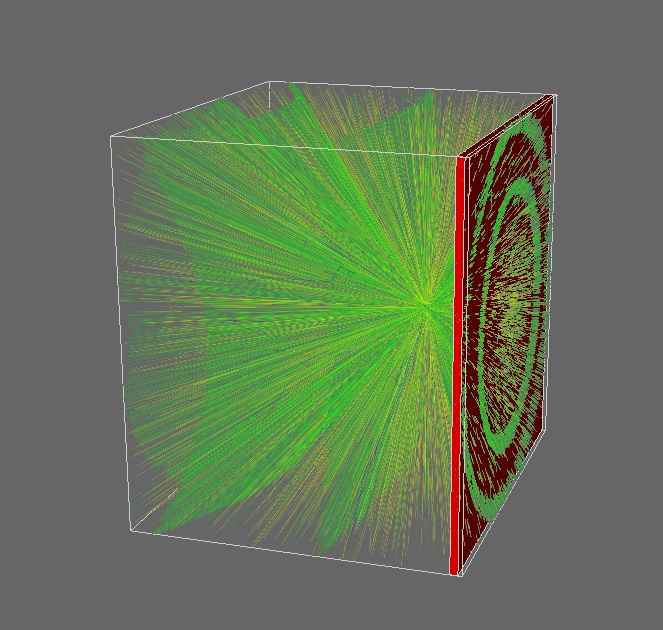
Which looks like neutrons are scattered in all directions. However, viewing the scene from far away (and increasing the statistics to 100k neutrons, just because), reveals how neutrons are scattered in nice Debye-Scherrer cones (because the sample is polycrystalline aluminium, modelled in the powder approximation):

For reference, here are the particle colours (they are also printed in the terminal):

Particle(s)	Colour
n	Green
\(\gamma\)	Yellow
\(e^-\)	Blue
\(\mathrm{p}\)	Red
\(\pi^\pm\)	Purple
\(\alpha\)	Cyan
Lithium-7	Orange
Others	White

Visualising generator aim

A very typical usage of the viewer is to debug whether the particle generator and the geometry are positioned correctly with respect to each other (if, say, half of the neutrons miss a detector by mistake, a less than careful analysis might conclude that the detector efficiency is about 50% too low!).

So one might, for instance, launch the viewer with 1000 neutrons (here is the BoronTube simulation from the dgcode_val bundle):

sb_borontube_sim -n1000 incidence_angle_deg=30 --dataviewer

It is clear that there is some sort of intense beam of neutrons passing through the test cell (the green tube in the center), but the picture is a bit messy. Instead, we have a special “generator aiming mode” of our viewer, in which only the primary (i.e. generated) particles are shown, and only the very first segment of each of those (to use Griff terminology). To use it, use the --aimdataviewer flag (or just --aim for short):

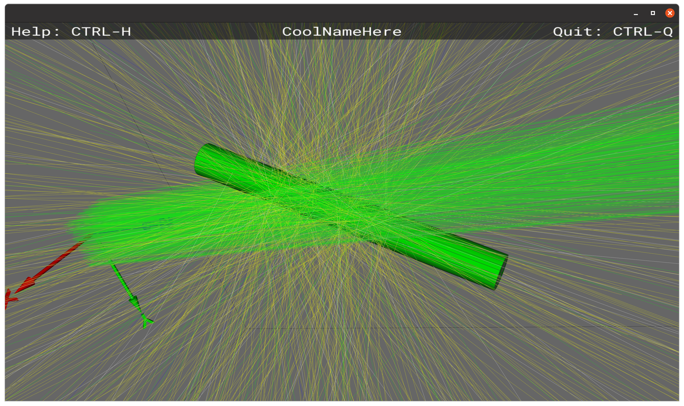
sb_borontube_sim -n1000 incidence_angle_deg=30 --aimdataviewer

And get:

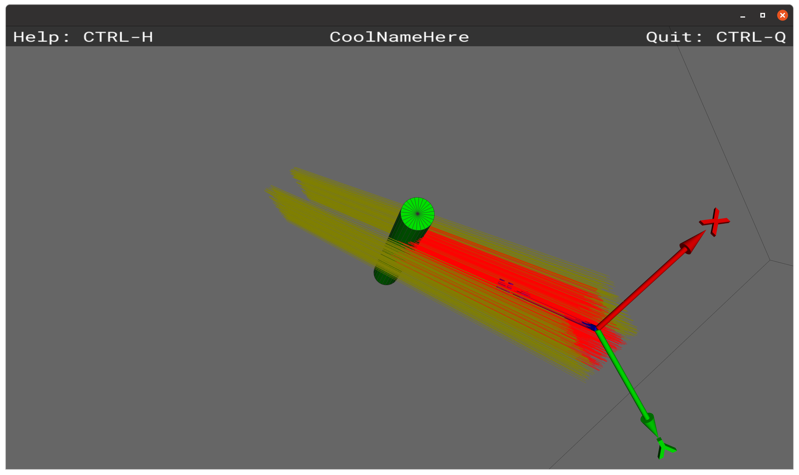
Now it is much more clear how our generated beam intersects the geometry. Especially since particles are no longer coloured as per their type in this mode, but rather coloured yellow if they never hit another volume than the one they start in, and red otherwise.

Visualising content of Griff file

It is possible to simply visualise the events inside a particular Griff file, by using the sb_g4osg_viewgriff command:

$> sb_g4osg_viewgriff -h
Usage:

  sb_g4osg_viewgriff [options] <Griff-file>

Display the simulated data (tracks) in the provided Griff file.

Options:

  -g, --loadgeo: Construct and display the geometry according to the meta-data
                 of the Griff file. WARNING: If the code changed since the griff
                 file was produced, the displayed geometry might different from
                 the one used while producing the Griff file!!!

  -e EVENTS: Only visualise certain events from the file, by specifying event
             indicies (i.e. positions in file: 0 is the first event, 99 is the
             100th event). The numbers can be provided either directly on the
             command line, or by specifying names of text files containing the
             numbers. Use commas to separate multiple entries.

So running sb_g4osg_viewgriff myfile.griff will visualise the tracks inside the file myfile.griff, and the -e flag can be used to pick out certain events only. Additionally, if the code in the geometry module did not change since the Griff file was produced, one can also use the -g flag to visualise the geometry as well. So sb_g4osg_viewgriff -g myfile.griff will visualise the tracks inside myfile.griff alongside the geometry. Crucially, this will use the geometry parameters that were actually used when myfile.griff was produced, and not their default values.

Environment variables

Admittedly the implementation could be improved, but as a solution for advanced users wanting to create some specialised plots, the following environment variables can be set in order to modify certain behaviours of the viewer (to be run in the terminal before invoking the command to launch the viewer):

• export G4OSG_BGWHITE=1 : Viewer will launch with a white background.

• export G4OSG_BGBLACK=1 : Viewer will launch with a black background.

• export G4OSG_NOWORLDWIREFRAME=1 : Don’t show the wireframe outline of the world volume at launch.

• export G4OSG_ENDTRACKSATVOL="MyVolumeName" : If a track crosses a volume with the given name, only the track parts until the volume will be shown.

• export G4OSG_TRKCOLALPHA=50 : All tracks will be 50% transparent (accepts number from 0..100).

• export G4OSG_TRKCOLR=100 G4OSG_TRKCOLB=0 G4OSG_TRKCOLG=0 : All tracks will be red (rgb value r=100%, g=0%, b=0%). Numbers must be in range 0..100.

• export G4OSG_SKIPSECONDARIES=1 : Only primary particles will be shown.

• export G4OSG_SCALEAXES=3 : Same as user doing 3 times Ctrl+up arrow (i.e. get bigger coordinate axes). Put to negative number to instead scale down.

Using Geant4’s own visualisation

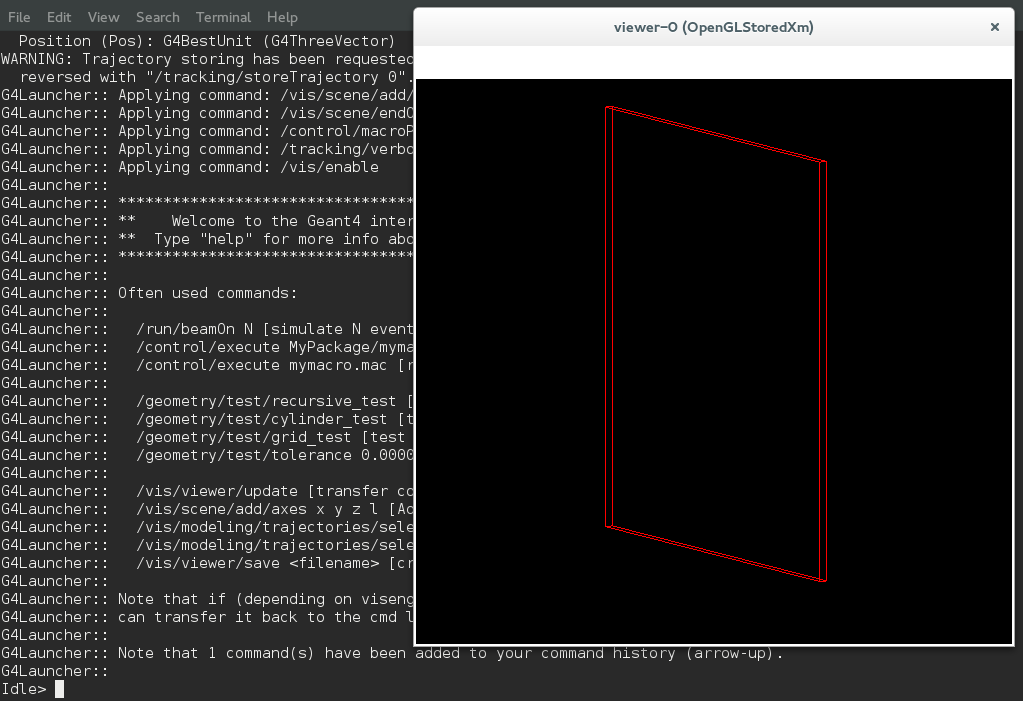
You can provide the flag -v to any simulation script to launch Geant4’s own visualisation option. Doing so will open a secondary visualisation window and drop you in a Geant4 interactive terminal which looks like this:

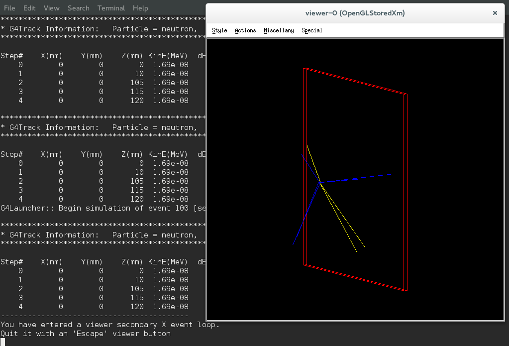
If you have problems, you can try using the -e option to select a different of the Geant4 drivers or “engines” (remember, you can see all the available options for the simulation scripts by supplying the option --help or -h). Upon startup, the visualisation window is completely unresponsive, and you have to switch control from the Geant4 terminal to the visualisation window by typing “/vis/viewer/update” or (to also simulate 10 events first) “/run/beamOn 10”. That leaves you with a view like the following:

Now, you can’t use the terminal again until you transfer control back there (from the menu Miscellany``→``Exit to G4Vis>). The Geant4 viewer is not really interactive as such, but you can change the viewing angle by using the menu “Actions”. It is beyond the scope of the present page to go further into the various commands that one might use in the interactive Geant4 terminal (which btw. can be opened without the visualisation window by the flag -i), except to note that a few of the more useful commands are printed by dgcode in the terminal (see first screenshot in this section), and refer interested parties to the official Geant4 documentation on visualisation.

Note that you exit the terminal by the command “exit” (or ctrl+D, like in BASH).