Performing parameter scans
It is very common that simulations and analyses need to be run for a variety of parameter settings (e.g. related to geometry and particle sources), before final conclusions can be drawn. In a simple case one might for instance, want to plot the value of some figure-of-merit as a function of a parameter (i.e. the thickness of some geometry volume, or the enrichment level of a particular material). Unfortunately, launching the relevant simulation and analysis jobs manually, while keeping track of both input parameters and output files, can be both tedious and error prone. To facilitate this process, dgcode provides ScanLauncher and ScanLoader utility classes in the ScanUtils package.
Important notice
The usage of the scanning utilities discussed here is of course completely optional, and might not be particularly helpful for all use cases. For one thing, the workflow discussed here is centered around analyses using Griff and SimpleHists for the work. Some users might prefer to implement their own custom solutions instead.
Users starting their project with the usual procedure for initialising a
new simulation project will already have three skeleton
scripts in the TriCorder package prepared which make use of these utilities, in
the scripts/simanachain, scripts/scan and scripts/scanana scripts
respectively. First we look at the script in the file
TriCorder/TriCorder/scripts/simanachain, which can be invoked with the name
sb_tricorder_simanachain. This simply combines the Geant4 simulation of the
sim-script with a Griff analysis running
on the output of the former, and creating a SimpleHists
file as a final result:
#!/usr/bin/env python3
import G4Utils.chain
G4Utils.chain.chain('sb_tricorder_sim','sb_tricorder_ana','REDUCED')
Any command line arguments provided to the sb_tricorder_simanachain command,
are simply passed on to the sb_tricorder_sim command.
Next, still in a project named TriCorder, one gets a scan script in the
file TriCorder/TriCorder/scripts/scan that can be launched with the command
sb_tricorder_scan. It has the contents:
from ScanUtils.ScanLauncher import ScanLauncher,ParameterGroup
from numpy import linspace

scan = ScanLauncher("sb_tricorder_simanachain",autoseed=True)
scan.add_global_parameter("rundir")
scan.add_global_parameter("--cleanup")
scan.add_global_parameter("--nevts",100000)
scan.add_global_parameter('--physlist','QGSP_BIC_HP_EMZ')
scan.add_global_parameter( 'material_lab',
                           'IdealGas:formula=CO2:pressure_atm=2.0' )

plot1 = ParameterGroup()
plot1.add('sample_radius_mm', linspace(1.0, 20.0, 5) )
plot1.add('neutron_wavelength_aangstrom', 2.2)
scan.add_job(plot1,'plot1')

plot2 = ParameterGroup()
plot2.add('sample_radius_mm', 5.0)
plot2.add('neutron_wavelength_aangstrom', [1.8, 2.2, 2.5] )
scan.add_job(plot2,'plot2')

scan.go()
We see here that, based on the sb_tricorder_simanachain command, several of
the sim-script parameters are provided with fixed values at
the top (including choice of physics list, some
material definitions, and that each job must model
\(10^5\) neutrons (a low value for purposes of having the skeleton example
run fast). After that, the actual jobs are defined in groups as desired. Here
two groups of parameter scans are defined and given names plot1 and
plot2, which indicates their ultimate intended usage for two particular
plots. Here, the first plot will vary the sample size while generating neutrons
of a constant wavelength, and the second plot will do the opposite and vary the
neutron wavelength while keeping the sample size constant (in a more realistic
scenario one would typically have more than just a handful of values of the
varied parameter).
The command sb_tricorder_scan --help provides full usage information, but if
one for instance wishes to launch the jobs locally with up to 16 concurrent
processes (i.e. on an 8-core machines with hyperthreading), one could for
instance run:
$> sb_tricorder_scan -qlocal -j16 -d ./my_scanresults --launch --halt-on-error
Next, one can analyse the results with the corresponding scanana script from
the file TriCorder/TriCorder/scripts/scan that can be launched with the
command sb_tricorder_scanana. It has the contents:
import ScanUtils.ScanLoader
import SimpleHistsUtils.cmphists
import sys
jobs=ScanUtils.ScanLoader.get_scan_jobs(sys.argv[1],dict_by_label=True)
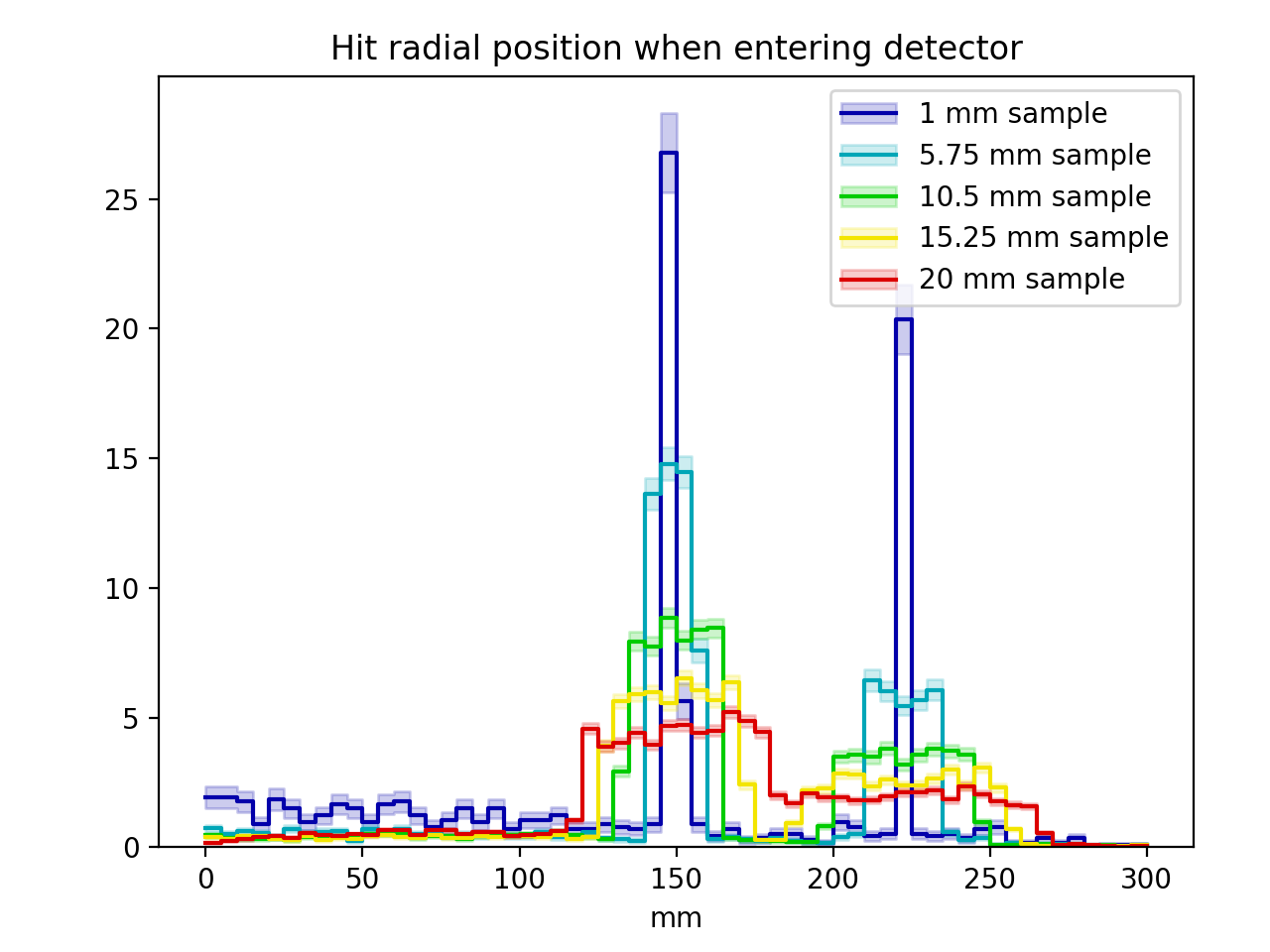
labelsandhists = [ ( '%g mm sample'%j.setup().geo().sample_radius_mm,
j.hist('det_hitradius') )
for j in jobs['plot1'] ]
SimpleHistsUtils.cmphists.cmphists( labelsandhists )
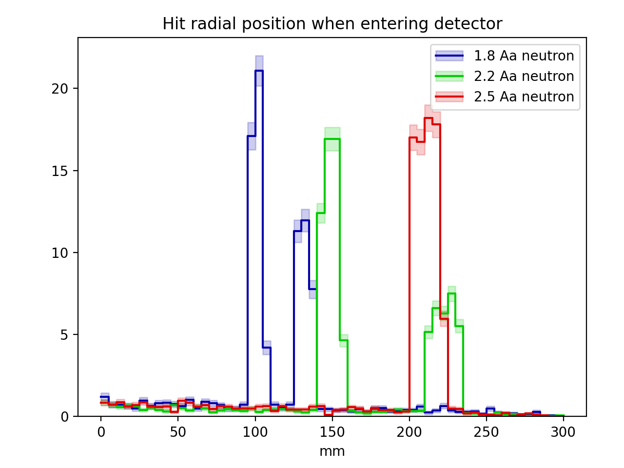
labelsandhists = [ ( '%g Aa neutron'%j.setup().gen().neutron_wavelength_aangstrom,
j.hist('det_hitradius') )
for j in jobs['plot2'] ]
SimpleHistsUtils.cmphists.cmphists( labelsandhists )
The most important line here is the one invoking get_scan_jobs(..), where
the results from the scan are loaded. This places the various histograms and
other metadata from the jobs into a dictionary, which allows easy plotting in
the following lines. In this simple example, a few histograms are simply
overlaid. In a more complicated example, one might instead perform some sort of
analysis of each job, in order to extract derived values, and so on, before
providing results.
In this example, the following two plots are produced. For those curious, they show how the Bragg reflections change as the neutron wavelength is changed, while the peaks around each Bragg edge are blurred by multiple-scattering effects if the sample size is increased.