SimpleHists

This page concerns our custom histogram solution for C++ and Python code, implemented as the simplebuild package SimpleHists.

Motivation

In addition to the obvious use cases of histograms (e.g. estimations of data probability density functions), histogram data types are also highly useful tools for data reduction, as they have a limited size in memory and on disk, no matter how much data is filled in them. Implemented correctly, they can even provide more functionality than just the counting of data-points in a certain binning. Examples include handling of errors, weights, and normalisations; collection of one-pass statistics such as unbinned mean and variance; association of metadata (title, axis labels); and utilities for on-disk storage and quick plotting.

Histogram classes are for instance found in the ROOT framework which is commonly used in high energy physics, but for Python-centric analyses based on tools like Numpy, SciPy, or Matplotlib, having a dependency on ROOT can be a bit onerous. However, one runs into the problem that e.g. Numpy does not by default include histogram classes. Rather, very basic histogramming functionality exists, but requires one to first collect all data into arrays, which, as mentioned, can give capacity issues for large data sets.

Features

The light-weight histogram classes, “SimpleHists”, provided in dgcode have several features that are all important to their usage in dgcode-based projects: usage from both C++ and Python, integration with Numpy and Matplotlib, persistification, quick plotting, extraction to Numpy arrays. Finally, the histograms have the crucial ability that data files collected in multiple concurrent jobs can be safely merged without the loss of any statistical metadata. More specifically, the list of features include:

Three feature-rich types of histograms: 1D, 2D and counter collection.
HistCollection which is an object representing a collection of histograms, each identified by a unique key.
- Such a collection class simplifies user code.
- Can be easily merged with other collections.
- Can be easily written to, or loaded from, a file (extension .shist).
Histograms themselves are also easily (de) serialisable:
- To/from raw bytes in both C++ and Python (in the form of std::string or bytes respectively).
- They work with the standard Python pickle module.
Histograms can be cloned, merged, normalised, scaled, integrated, …
The C++ interface is simple to use and very fast.
The Python interface additionally features integration with Numpy arrays and Matplotlib plotting.
Several command-line scripts for working with .shist files are available, supply --help to any of them for more detailed instructions:
- sb_simplehists_browse: Open up graphical browser.
- sb_simplehists_merge: Merge contents in two .shist files into one. This is meant as an easy and reliable way to merge output done in concurrent computing situations (such as at a computing cluster).
- sb_simplehists_extract: Extract a subset of histograms from a file into a smaller one.
- sb_simplehists2root_convertfile: For compatibility, convert histograms in a .shist file to ROOT histograms and store them in a .root file. This requires ROOT to have been installed in the environment, which might not be simple.

Example: Producing histograms in C++

Imagine for instance the following to be part of some big event loop running on a cluster, collecting histograms in a large number of jobs:

SimpleHists::HistCollection hc;
auto h_edep = hc.book1D("Energy deposited in counting gas",100,0.0,2000,"edep");
h_edep->setXLabel("keV");
auto h_scatterpos = hc.book2D("Scatter coordinates",100,0.0,2.0,100,0.0,2.0,"scatterpos");
h_scatterpos->setXLabel("depth [meters]");
h_scatterpos->setXLabel("height [meters]");
//Some big loop:
for (unsigned ievt=0; ievt < bignum; ++ievt) {
  // ...
  // All sorts of expensive stuff, for instance related to Geant4 simulations.
  // ...
  h_edep->fill(edep);
  h_scatterpos->fill(particle.x(),particle.y());
  // ...
}
hc.saveToFile("results.shist");

Afterwards, one can then use the sb_simplehists_merge command to merge the result.shist files from many different cluster jobs into one. Thus, relevant data from many billions and billions of events are now all present in a single small (tens of kilobytes) file which can be copied easily down to ones laptop for subsequent analysis. Of course, before launching computationally intensive jobs on a cluster, you will most likely have been running the same code on your own machine, while developing and verifying it.

Example: Python analysis of histograms

After having copied down the results.shist file to your laptop, the first thing to do is to have a quick look inside. This is done by the command:

$> sb_simplehists_browse results.shist

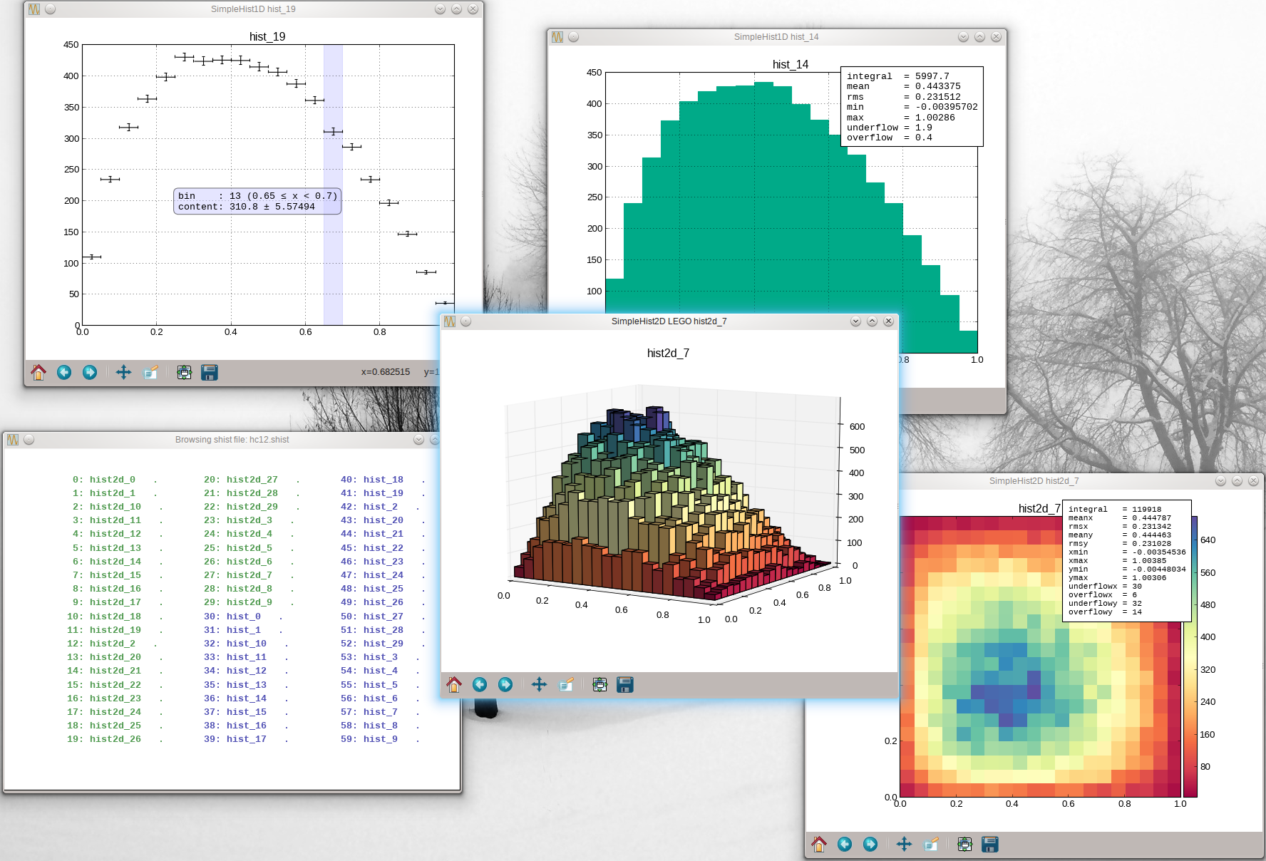
This opens up a graphical browser which can be used to quickly view the histograms with various options for the presentations. At this stage it is already possible to produce a few quick plots for a paper, talk or email.

For more advanced analysis, one can use Python and the plethora of utilities available there (e.g. all the utilities available in Matplotlib and SciPy). Here is a small example of how one can get data out in formats ready to input to various Matplotlib plotting routines:

import SimpleHists as sh
hc = sh.HistCollection('results.shist')
h_edep = hc.hist('edep')
#One can launch the quick interactive view for this histogram by:
h_edep.plot()
#But for advanced customised analysis and plotting, you can ask for the
#contents and bin edges in the same format as numpy.histogram(..) would
#return:
contents, edges = h_edep.histogram()
#This can be used for custom analysis (using SciPy fitting/interpolation
#tools, making plots with analytical results on top, etc., etc.)
#One can access other statistics as well of course:
print('edep variance =', h_edep.rms)
print('mean edep     =', h_edep.mean)